I probably shouldn’t have, but it was fun.

Anyway, all you flat-earthers, here are the implications of your model. I am well aware that, in today’s world, proving something with ironclad logic and granitic certainty is useless as regards changing anybody’s mind. However, like Don Quixote, once in a while I tilt at windmills. I list here and illustrate ‘where the sun is’ in the sky for a flat earth model. I provide the (python) code for calculating what I show, and I also give tables of sky coordinates. It’s my own mini Rudolphine Tables!

Background

Most variants of the flat earth model resemble Rowbotham’s 1849 one. In this model, the north pole is in the center of the disk, and south is always outward. There’s an edge, or, in some models, an ice wall, at the perimeter of the circle. The equator is a circle (roughly) 10,000 km in radius, centered on the north pole. The stars inhabit a disk about 5000 km above the ground, and this starry disk rotates at the steady pace of about one spin per day.

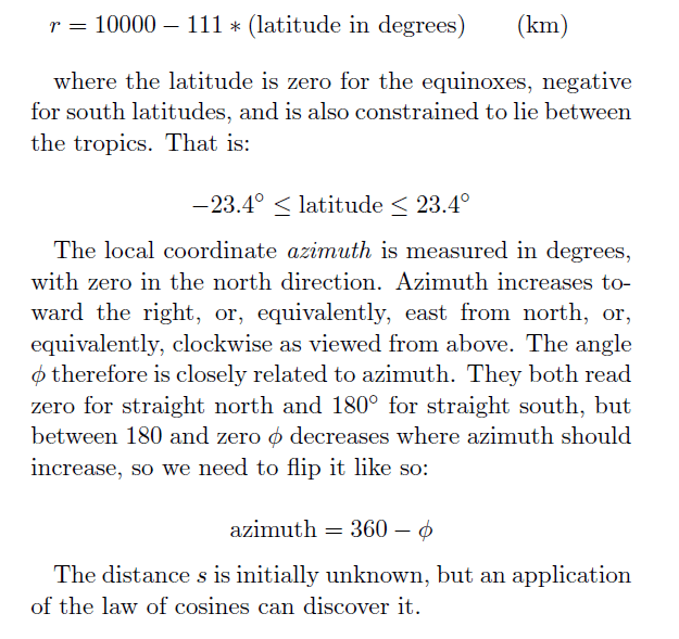
The sun is at 4800 km height (i.e., closer than the stars by a little bit). The solar orb also rotates about once a day. At the equinoxes, its radial distance from the rotation axis is 10,000 km. At the June solstice, it is above the Tropic of Capricorn at 23.5 degrees north latitude, or a radial distance of 10000 – 2600 = 7400 km. At the December solstice, the sun is above the Tropic of Cancer at 23.5 degrees south latitude, or a radial distance of 10000 + 2600 = 12600 km from the rotation axis.

Latitude and longitude are earth-location coordinates. Latitude is the north-south coordinate. By convention, Latitude is zero at the equator, 90 degrees at the north pole, and “negative” 90 or “90 degrees south” at the south pole (or, in the flat earth model, at the edge of the disk). Longitude is the round-and-round coordinate. The location of longitude = 0 is arbitrary, but since 1884 the convention has been to use England’s Greenwich Observatory as the zero point. Longitudes are measured east or west from this prime meridian. The 180 degree east = 180 degree west meridian is the approximate location of the international date line.

The French initially defined the meter as 1/10,000,000 the distance from the north pole to the equator. Hence, the 10,000 km number (for the north pole to equator distance) is actually correct and only slightly rounded. Sideways (east-west) distances differ between flat earth and round earth models. Let’s say that delta lambda is the longitude difference between two observers and phi is the latitude (and the observers have the same latitude). To a few tenths of a percent accuracy for the round earth, the east-west distance is M_r * (delta lambda in radians) * cos(phi), where M_r is 6,367,449 meters, the “mean meridional radius” of the earth. In the flat earth picture, the east-west distance is (delta lambda in radians) * (north pole to observer distance). The two methods diverge strongly in the southern hemisphere all the way to the absurd south pole situation, where all east-west distances are zero for a round earth, but to circumnavigate the ice wall would be to travel 2*pi*20,000 km = 125,664 km.

One more piece of background: the last one, I swear. Altitude and azimuth are local coordinates, by which I mean unique to each observer located on the surface of the earth. Local coordinates include the N, E, S, W cardinal directions, the zenith (straight up), and the nadir (straight down). Different observers will in principle measure different local coordinates for a given sky event. Azimuth is the round-and-round coordinate, starting with zero in the north direction. From the zero point, mark off angles to the right, in degrees, so that east is 90 degrees azimuth, south is 180 degrees azimuth, and west is 270 degrees azimuth. 360 degrees turns back into zero. Altitude is the angle from the horizon up to the sky object. The maximum altitude is 90 degrees, also known as zenith. The minimum altitude is negative 90, the nadir, straight down into the ground.

The question “where is the sun?” is answered by using altitude and azimuth. Reminder: altitude and azimuth are local coordinates, unique to a given observer.

Flat Earth Geometry

Here is a top view of the Robotham flat earth.

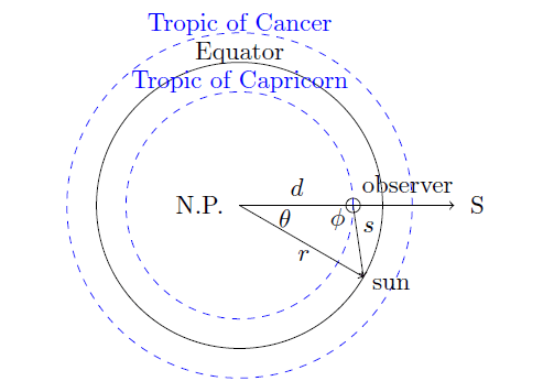
The triangle vertex marked “N.P.” is the north pole. The distance from the north pole to the observer is “d,” and that observer’s south compass direction is marked “S.” The distance “r” is the radial-only distance from the north pole to the sun (we’ll include the sun’s height later). The sun distance that is illustrated is 10,000 km, from the N.P. to the equator, but the sun’s distance can vary seasonally between the tropic circles. The angle theta can be calculated via the time since noon.

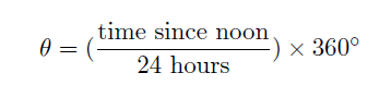
The “noon” whereof we speak is local noon for the particular observer. The sun is highest in the sky at this moment, and also located at the observer’s 0-azimuth or 180-azimuth, depending on if “d” is greater than or less than “r.” Note that

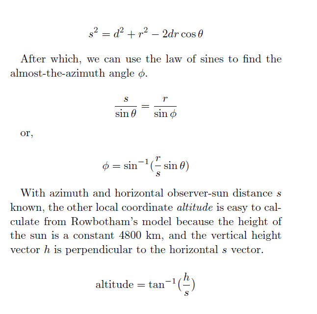
Success. That’s how to calculate azimuth and altitude from the Rowbotham model from known quantities (time of day, season, and observer’s distance from the north pole).

Graph that up with a little Python Script

import numpy as np
import math
from pylab import *


# script to compute Azimuth and Altitude for the sun
# in the Rowbotham flat earth model. Assumptions:
# 1. The sun is at 4800 km height.
# 2. The sky and earth have a relative rotation which is steady
#    at 360 degrees per day
# 3. The pole to equator distance is 10,001.96 km, so it's 20,003.92 km
#    from the north pole to the Rowbotham edge, or ice wall.
#
# For comparison, also shows the Greek celestial sphere az, alt
# Approximates the sun's seasonal drift with a sin function of the
# proper amplitude (2600 km or 23.4 degrees).
# Output: a plot of az vs. alt and a .csv table of az and alt as function of
# time since local noon, for one observer.
#
# Constants:
h = 4800.0 # km, for the sun (stars are at 5000 km)
degrad = 180.0/math.pi
arraylen = 400

# User inputs, two of them:
# User's distance from the north pole:
d = 12600  # km
# Date: fraction of one year since equinox (for seasonal drift)
# I.e., spring equinox = 0, June solstice = 0.25, fall equ = 0.5, Dec sol = 0.75
date = 0.75  # unitless

#
# Rowbotham
#

# Pack 'time since noon' into an array
delt = 1.0e-10 # li'l fudge for starting and ending. Units: hours
timesincenoon = np.linspace(-12.0+delt,12.0-delt,num=arraylen) # hours

# calculated quantities
# Radial distance of sun from north pole
sundist = 10001.96 - 2600.0*np.sin(date*2.0*np.pi)  # km
# hour angle-ish thing (theta)
theta = (timesincenoon/24.0)*2.0*np.pi # radians
# observer-sun horizontal distance
s = np.sqrt(d**2 + sundist**2 - 2.0*d*sundist*np.cos(theta))  # km
# angle related to the azimuth
phi = np.asin( (sundist/s)*np.sin(theta))  # radians
# For the morning half of the circle, flip the sign of phi
for i in range(len(theta)):
    if (theta[i] > math.pi) or (theta[i] < 0.0):
        phi[i] = -phi[i]
# phi's quadrant may be ambiguous. Apply a test compared to a right triangle.
# sundist^2 = d^2 + s^2 for a right triangle.
# sundist^2  d^2 + s^2 for obtuse phi
for i in range(arraylen):
    if (sundist**2) > (s[i]**2 + d**2):
        phi[i] = math.pi - phi[i]

# azimuth
az = np.zeros(arraylen,dtype=float)
for i in range(len(theta)):
    if theta[i] > 0.0:
        az[i] = 2.0*np.pi - phi[i]
    else:
        az[i] = phi[i]  # radians
alt = np.atan(h/s)

#
# Greek
#

# now, include the "round earth" solar az-alt calculation
sundec = (23.4/degrad)*np.sin(date*2.0*np.pi) # radians
delt = delt*15.0/degrad
ha = np.linspace(-1.0*math.pi+delt,math.pi-delt,num=arraylen)  # hour angle, in radians
# note that HA might be increasing to the east. 
latitude =(math.pi/2.0)* ((10001.96 - d)/10001.96 ) # radians

print('sun dec, observer latitude =',sundec*degrad,latitude*degrad)

saz = np.atan2(np.sin(ha),np.cos(ha)*np.sin(latitude) - np.tan(sundec)*np.cos(latitude) )
saz = saz + np.pi

salt = np.asin(np.sin(latitude)*np.sin(sundec)  + np.cos(latitude)*np.cos(sundec)*np.cos(-ha) )

print('at midnight az, alt =',saz[0],salt[0])
nq = int(arraylen/2) -1

# estimate the two sets of angular velocities (just do a backwards difference - very crude)
#   (also, assume small angles, itself a decently safe assumption) 
dadt = np.zeros(arraylen,dtype=float);sdadt = np.zeros(arraylen,dtype=float)
for i in range(1,arraylen):
    deltat = timesincenoon[i]-timesincenoon[i-1]
    dadt[i] = math.sqrt(((az[i]-az[i-1])*math.cos(alt[i]))**2+(alt[i]-alt[i-1])**2)/deltat
    sdadt[i] = math.sqrt(((saz[i]-saz[i-1])*math.cos(salt[i]))**2+(salt[i]-salt[i-1])**2)/deltat
# Now for the entry that straddles midnight.
# This is tricky because it might be near Az=180 or it might be near Az=0=360
deltat = 24.0 - (timesincenoon[-1] - timesincenoon[0]) # the bit of time between last and first array entry
if ( abs(math.pi - az[0]) < 1.0):
    dadt[0] = math.sqrt(( ((az[-1]-az[0]))*math.cos(alt[0]))**2+(alt[-1]-alt[0])**2)/deltat  # radians per hour
else:
    dadt[0] = math.sqrt(( (2.0*math.pi - (az[-1]-az[0]))*math.cos(alt[0]))**2+(alt[-1]-alt[0])**2)/deltat  # radians per hour
    
deltat = (degrad/15.0)*(2.0*math.pi - (ha[-1] - ha[0]))
if ( abs(math.pi - saz[0]) < 1.0):
    sdadt[0] = math.sqrt((((saz[-1]-saz[0]))*math.cos(salt[0]))**2+(salt[0]-salt[-1])**2)/deltat # radians per hour
else:
    sdadt[0] = math.sqrt(((2.0*math.pi - (saz[-1]-saz[0]))*math.cos(salt[0]))**2+(salt[0]-salt[-1])**2)/deltat # radians per hour
     

print(timesincenoon[0],timesincenoon[-1],24.0 - (timesincenoon[-1] - timesincenoon[0]),(degrad/15.0)*(2.0*math.pi - (ha[-1] - ha[0])))
print(az[-1],az[0],alt[-1],alt[0],az[-1]-az[0],alt[-1]-alt[0],'radians')
print(saz[-1],saz[0],salt[-1],salt[0],saz[-1]-saz[0],salt[-1]-salt[0],'radians')


      
plot(az[0:nq]*degrad,alt[0:nq]*degrad,color='xkcd:aqua',label='Rowbotham')
plot(az[nq+1:-1]*degrad,alt[nq+1:-1]*degrad,color='xkcd:aqua')
plot(saz[0:nq]*degrad,salt[0:nq]*degrad,color='xkcd:brick red',label='Greek')
plot(saz[nq+1:-1]*degrad,salt[nq+1:-1]*degrad,color='xkcd:brick red')
plot([0,360],[0,0],'k')
plot([180,180],[0,5],'k')
text(180,6,'S',ha='center')
plot([270,270],[0,5],'k')
text(270,6,'W',ha='center')
plot([90,90],[0,5],'k')
text(90,6,'E',ha='center')
plot([0,0],[0,5],'k')
text(0,6,'N',ha='center')
plot([360,360],[0,5],'k')
text(360,6,'N',ha='center')

ip=np.searchsorted(timesincenoon,-9.0)
text(degrad*az[ip],degrad*alt[ip],'3 a.m.',ha='center',va='center',color='xkcd:aqua')
ip=np.searchsorted(timesincenoon,-6.0)
text(degrad*az[ip],degrad*alt[ip],'6 a.m.',ha='center',va='center',color='xkcd:aqua')
ip=np.searchsorted(timesincenoon,-3.0)
text(degrad*az[ip],degrad*alt[ip],'9 a.m.',ha='center',va='center',color='xkcd:aqua')
ip=np.searchsorted(timesincenoon,0.0)
text(degrad*az[ip],degrad*alt[ip],'noon',ha='center',va='center',color='xkcd:aqua')
ip=np.searchsorted(timesincenoon,3.0)
text(degrad*az[ip],degrad*alt[ip],'3 p.m.',ha='center',va='center',color='xkcd:aqua')
ip=np.searchsorted(timesincenoon,6.0)
text(degrad*az[ip],degrad*alt[ip],'6 p.m.',ha='center',va='center',color='xkcd:aqua')
ip=np.searchsorted(timesincenoon,9.0)
text(degrad*az[ip],degrad*alt[ip],'9 p.m.',ha='center',va='center',color='xkcd:aqua')

#text(degrad*saz[0],degrad*salt[0],'midnight',ha='center',color='xkcd:brick red')
ip = np.searchsorted(ha,-np.pi*(3/4))
text(degrad*saz[ip],degrad*salt[ip],'3 a.m.',ha='center',va='center',color='xkcd:brick red')
ip = np.searchsorted(ha,-np.pi*(2/4))
text(degrad*saz[ip],degrad*salt[ip],'6 a.m.',ha='center',va='center',color='xkcd:brick red')
ip = np.searchsorted(ha,-np.pi*(1/4))
text(degrad*saz[ip],degrad*salt[ip],'9 a.m.',ha='center',va='center',color='xkcd:brick red')
ip = np.searchsorted(ha,0.0)
text(degrad*saz[ip],degrad*salt[ip],'noon',ha='center',va='center',color='xkcd:brick red')
ip = np.searchsorted(ha,np.pi*(1/4))
text(degrad*saz[ip],degrad*salt[ip],'3 p.m.',ha='center',va='center',color='xkcd:brick red')
ip = np.searchsorted(ha,np.pi*(2/4))
text(degrad*saz[ip],degrad*salt[ip],'6 p.m.',ha='center',va='center',color='xkcd:brick red')
ip = np.searchsorted(ha,np.pi*(3/4))
text(degrad*saz[ip],degrad*salt[ip],'9 p.m.',ha='center',va='center',color='xkcd:brick red')

xlabel('Azimuth')
ylabel('Altitude')
legend(frameon=False)
title('Sun local coordinates. Observer is '+str(d)+' km S of north pole.')
show()


# To do: angular velocity calculation
#        output a csv file
import csv

tag=str(int(d)).zfill(5)  # label file by the polar distance number
with open('altaz_d'+tag+'.csv','w') as csvfile:
    cwriter = csv.writer(csvfile,quoting=csv.QUOTE_MINIMAL)
    cwriter.writerow(['Time (h)','Rowb Az (deg)','Rowb Alt (deg)','dA/dt','Grk Az (deg)','Grk Alt (deg)','dA/dt'])
    for i in range(arraylen):
        cwriter.writerow([timesincenoon[i],degrad*az[i],degrad*alt[i],degrad*dadt[i],degrad*saz[i],degrad*salt[i],degrad*sdadt[i]])

I cannot tell a lie: The hardest thing about coding up the above equations was dealing with the sunrise side versus the sunset side of things.

So. Where is the sun, then?

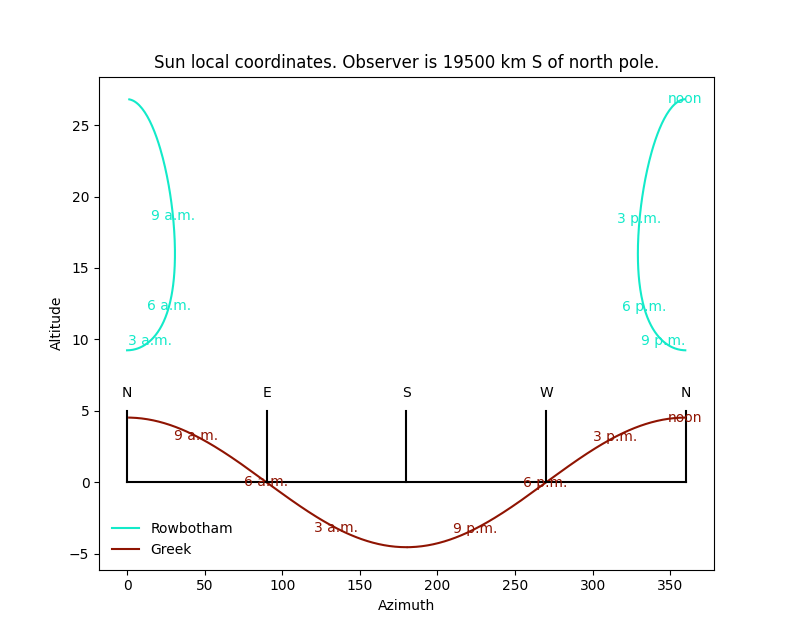
Let’s place the sun at equinox, so that it’s over the equator at noon (in both models). In the series of graphs that follow, we plot altitude versus azimuth for different observers, starting near the north pole and working our way south. “Greek” refers to the spherical earth model that has been in the historical record for about 2500 years. I ignore oblateness and other subtleties that may cause fractions-of-a-percent corrections. As the first graph should serve to show, the divergence between flat earth and round earth predictions are massive (e.g., over 500% for noon altitude of the sun).

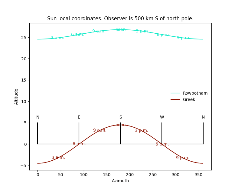
In the Greek picture, the sun is less than 5 degrees from the horizon at noon, then sets due west. In the Rowbotham model, the sun is about 25 degrees from the horizon and basically circles around us like a vulture. I guess at some point, the sun will wink out due to its supposed lampshade, but I have no idea how to make a physical model of that. In the pictures, negative altitudes simply mean that the sun is below the horizon. This only occurs in the Greek picture, of course.

Greek: The noon sun is 23.4 degrees above the horizon at noon and sets due west. Flat: the sun winks out (6pm) while about 25 degrees up.

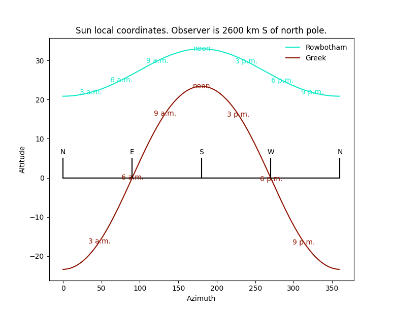
At mid-latitudes, i.e., close to where Rowbotham lived, the sun’s altitude at noon is the same in both models. However, the sun is still higher than 20 degrees when it winks out in the flat earth picture.

Similar to the previous graph, but the flat earth sun gets lower in the sky before winking out.

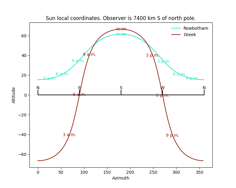
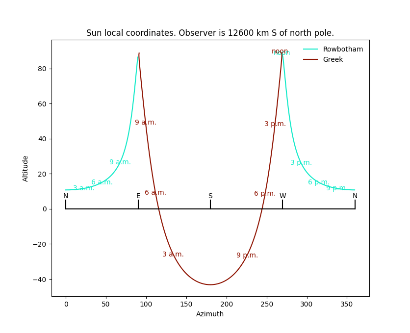
This figure (once seen I can’t unsee it) looks like a Kilroy Was Here doodle. It has gone wonky because we are now south of the equator. The noon sun is closer to the north horizon than the south horizon. It’s still equinox, so it rises due east and sets due west. One could easily replot this to put north in the middle of the graph, but I didn’t, to keep things consistent. The flat earth sun now follows a distorted oval in the northern sky between plus and minus 55 degrees azimuth, give or take, and never approaching the required plus and minus 90 degrees.

In the Greek picture, the sun still sets due west and, in a mirror of what happens in the north, rises to less than 5 degrees off the horizon at noon. The flat earth picture now has a sun making a more and more distant circle, now contained within plus or minus 30 degrees from due north, more or less. This is entirely different from its behavior in the first of this series of figures, where it circled the observer and covered all azimuth angles.

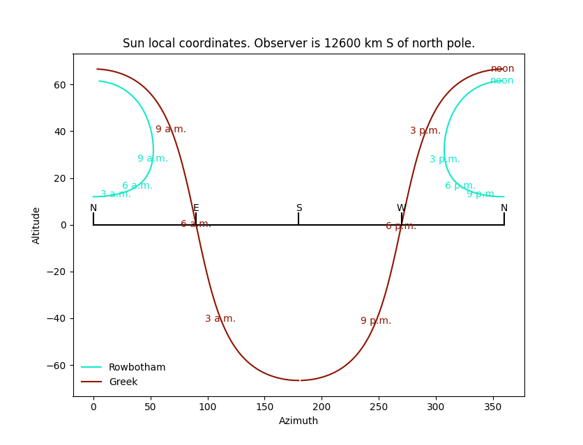
I have one more fun picture for you. Suppose you are located at the Tropic of Cancer, but it’s December 21, so that the noon sun is directly overhead. The diagram you get is a head-scratcher at first. Let me show you.

Firstly, in both pictures, there is a massive skip between a minute before noon to a minute after noon. That’s because the sun passes overhead. So, one minute it’s climbing the eastern sky and then in the next minute it’s descending the western azimuth line. This is to be expected, if you think about it for a minute.

Secondly, I love the split behavior. The Rowbotham sun trends north after noon, while the Greek sun trends to the south. (So, talk to somebody that lives in Tonga. They could plant a vertical stick in the ground to make a shadow observatory and make an azimuth circle around the stick. Next December solstice, et voila!, we’d finally know which model is correct.) Because we are no longer at equinox, there are more daylight hours than nighttime hours in the Greek picture.

For an Excel sheet with the data used to plot the above graphs, click here. (It contains the data from the csv files that the python program outputs.) As a bonus extra, I also computed (roughly) the angular velocity of the sun across the sky in both models (for the Greek model, the angular velocity is constant, so the extent that my rough calculation deviates from constancy is a measure of the accuracy of the calculation, and it’s about 1%.)

Conclusion

There. Done. The python program can be easily changed for different-sized disks or different solar altitudes. That is, any flat earth model that vaguely resembles the Rowbotham one can be accommodated. So, there you go, flat-earthers: here are the geometrical consequences of the most popular flat earth model.

Now go buy a theodolite and go measure stuff!

(Bet nobody will. Sigh.)